
Table of Contents
Summary
Fiber-reinforced plastics can consist of a combination of individual layers to form a multilayer composite. With unidirectional layers, different stress profiles result depending on the load case and orientation of the layers. The problem addressed here is determining the orientation of each individual layer in order to achieve optimal utilization of the multilayer composite. This is an optimization problem for which a systematic solution is developed here. To this end, an overview of similar studies in the literature is first provided, in which different nature-inspired optimization methods were used. Then, the Evolution Strategy is selected and applied to the problem at hand. Parameter studies are carried out to determine correlations in terms of performance and result quality. These then serve as a basis for investigating underlying regularities.
Introduction
Fiber-reinforced plastics (FRP) are modern materials that are used in a wide range of products and components. Now that the potential of steels and other metal alloys has gradually been exhausted, great hopes are being placed in this relatively young technology. Excellent weight-specific properties such as strength and stiffness make them ideal for achieving significant weight savings. At the same time, however, FRPs are also more sensitive in many respects and derive their load-bearing capacity from principles that are completely different from those of metals. This presents both opportunities and challenges. The biggest difference is that loads can basically only be absorbed by the fibers; the surrounding plastic is relatively weak and has other functions.
This is most evident in so-called unidirectionally reinforced fabrics, or UD fabrics for short. These are thin flat structures, called laminates or single layers, whose continuous fibers lie in only one direction and can therefore only absorb significant loads in one direction. Such layers are arranged on top of each other and used as a multi-layer composite (hereinafter also referred to as “laminate”). In view of the load, the boundary conditions, and all other design parameters, which can vary greatly depending on the application, the question now arises as to how the layers should be arranged in order to obtain the required property profile for the application — an optimization problem.
Deterministic optimization methods such as the simplex algorithm sometimes converge (too) early to a local optimum. In order to get as close as possible to the actual optimum, however, a promising approach is to use nature-inspired, heuristic optimization methods. Even with a large number of parameters and difficult objective functions (e.g., non-convex, discontinuous, etc.), they can determine optimal solutions with a high degree of probability. However, the decisive factor here is how the input parameters of the algorithm are selected so that it performs well, i.e., delivers these results efficiently and reliably.
This study deals with the selection of a suitable optimization algorithm, its application to laminates with different numbers of individual layers, the handling of input parameters, and the evaluation of results.
Classical laminate theory
The laminate model consists of any number of unidirectional layers arranged one above the other, in this case layers of glass fiber reinforced plastic (GRP). The characteristic values used here are listed in Table 1. For the individual layers, a plane stress state is assumed, which means that stresses in the direction of the thickness per layer are neglected, i.e., they are considered as discs/plates with stresses occurring in the plane. Therefore, σz=τzx=τyz=0 applies. The basic stresses are therefore tension in the fiber direction, tension transverse to the fiber direction, and shear in the plane. Influences from the manufacturing process, such as bonding, material inhomogeneities, or differing fiber contents, are neglected. This is therefore an idealized model.
The Kirchhoff-Love disc/plate theory is illustrated here. With regard to classical laminate theory, it describes the following assumptions:
- The plate thickness is small compared to the other geometric dimensions.
- The deflection of the plate is small compared to its thickness, and the inclinations are small compared to one.
- Straight line segments that were originally orthogonal to the central surface remain straight and orthogonal to the deformed central surface even in the deformed state (distortions are distributed linearly across the plate thickness).
- The stresses σz normal to the central surface (MF) can be neglected.
- There is complete adhesion between the individual layers (idealized composite).
| E1 (MPa) | E2 (MPa) | ν12 | ν21 | G12 (MPa) | Thickness (mm) |
|---|---|---|---|---|---|
| 44500 | 12500 | 0,28 | ν12 ∙ E2/E1 | 6000 | 0,2 |
The calculations of the stresses in each individual layer, which can be derived from the laminate load, can be summarized in the following steps:
First, the four independent material parameters of each layer, which result from their transversely isotropic mechanical properties, are determined by applying micromechanical models, conducting experiments, or taking them from the literature. This allows the so-called “local” stiffness matrix to be established for each layer, in which the 1-direction indicates the fiber direction and the 2-direction indicates the direction perpendicular to the fiber direction. The stiffness matrix is therefore:
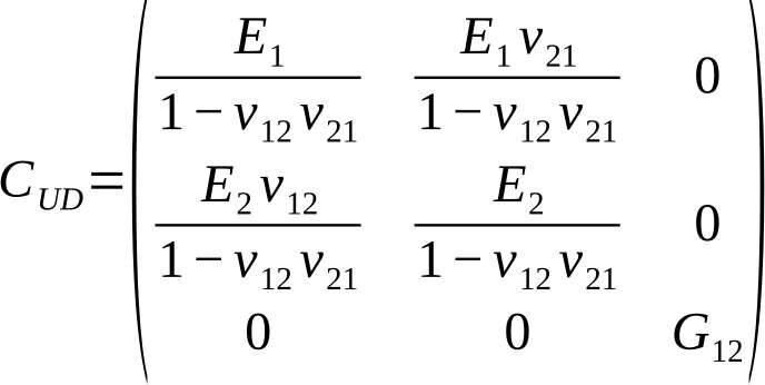
The stress-strain relationship according to Hooke’s law is given by
σUD=CUD ∙ εUD:

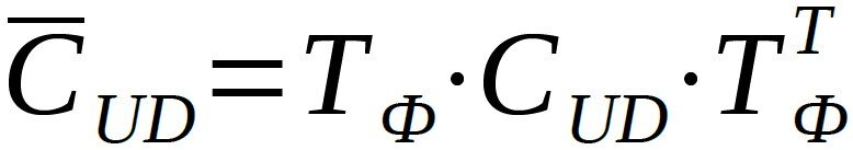
The stiffness relationships for each layer are hereby described in relation to their local coordinate systems. The next step is to convert them into a global coordinate system for the composite. This is done using the transformation matrix TФ:
The transformation is being described with:
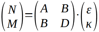
This completes the description of the stress-strain relationship of the layers and their rotation in a common, global coordinate system. Subsequently, the so-called ABD matrix is established using the static equilibrium conditions, which expresses the relationships between internal forces (force and moment flows) and the strains and curvatures of the laminate. The name comes from the fact that this matrix consists of four 3×3 matrices, namely one A-matrix representing the properties of the disc, one D-matrix representing the properties of the plate, and two B-matrices describing the coupling of shear forces and moments or strains and curvatures. With N for the shear forces, M for the shear moments, ε for the strains, and κ for the curvatures, this relationship results in:
Once the shear forces have been determined from the static equilibrium, the global strains and then the global stresses can be calculated. These are then transformed back to determine the prevailing stresses in the respective layer coordinate system. Failure criteria can then be applied to evaluate the strength of a laminate and determine its acceptability. For details on classical laminate theory and its derivation, see [1].
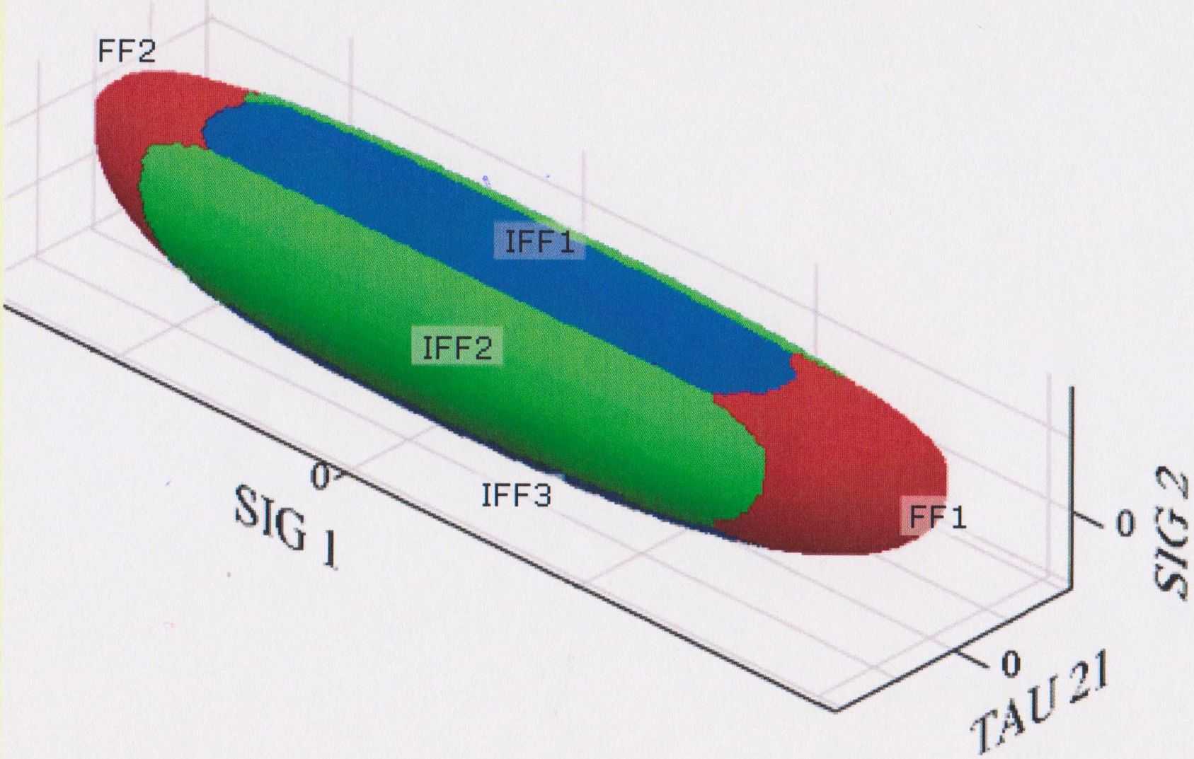
CUNTZE failure criteria
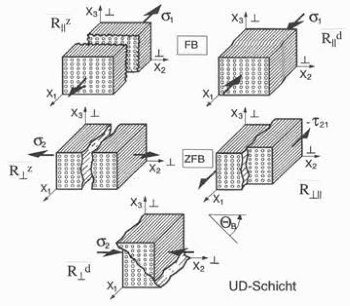
The failure criterion according to CUNTZE (for details, see [2]) with its described Failure Mode Concept will be applied in this work. It distinguishes failure by five different failure modes, namely:
- Fiber failure („FB“ resp. „FF“) with
- Tensile stress along the fiber R||z
- Compressive stress along the fiber R||d
- interfiber fracture („ZFB“ resp. „IFF“) with
- Tensile stress perpendicular to the fiber direction R⊥z
- Compressive stress perpendicular to the fiber direction R⊥d
- Shear stress along the fiber direction R⊥||
There are basically two different approaches to defining when failure occurs, namely first-ply failure and progressive failure. In first-ply failure, failure occurs when one ply of the laminate loses its load-bearing capacity. The laminate then retains its residual strength or stiffness. In progressive failure, failure occurs when the last individual ply has also lost its load-bearing capacity. The first-ply failure approach is applied here.
Nature-inspired optimization of composites: status today
First, an overview is provided of how fiber-reinforced plastics are optimized using nature-inspired methods. Of particular interest here is the frequency with which certain algorithms were used. The question that arises is whether a pattern can be identified behind the frequency of the specific optimization goal and the algorithms used for this purpose. In addition, we will examine whether conclusions can be drawn from this regarding the thesis that there is a suitable algorithm for every optimization goal applied to FRP.
The databases and search engines used to search for scientific publications on the Internet are www.Scopus.com and www.ScienceDirect.com. These are searched using the following optimization algorithms:
- Genetic Algorithm (GA)
- Evolution Strategy (ES)
- Particle Swarm Optimization (PSO)
- Ant Colony Optimization (ACO)
- Artificial Bee Colony (ABC)
- Artificial Immune System (AIS)
Publications are searched for and collected by combining keywords such as “laminate, CFRP, lay-up, stacking sequence, composite, fiber reinforced, optimization, evolutionary optimization, evolutionary algorithm, nature-inspired, bio-inspired, ant colony, particle swarm,” etc. The publications are then sorted, first according to their optimization goal and then according to the algorithm used. Multi-objective optimization is treated separately, but according to the same pattern.
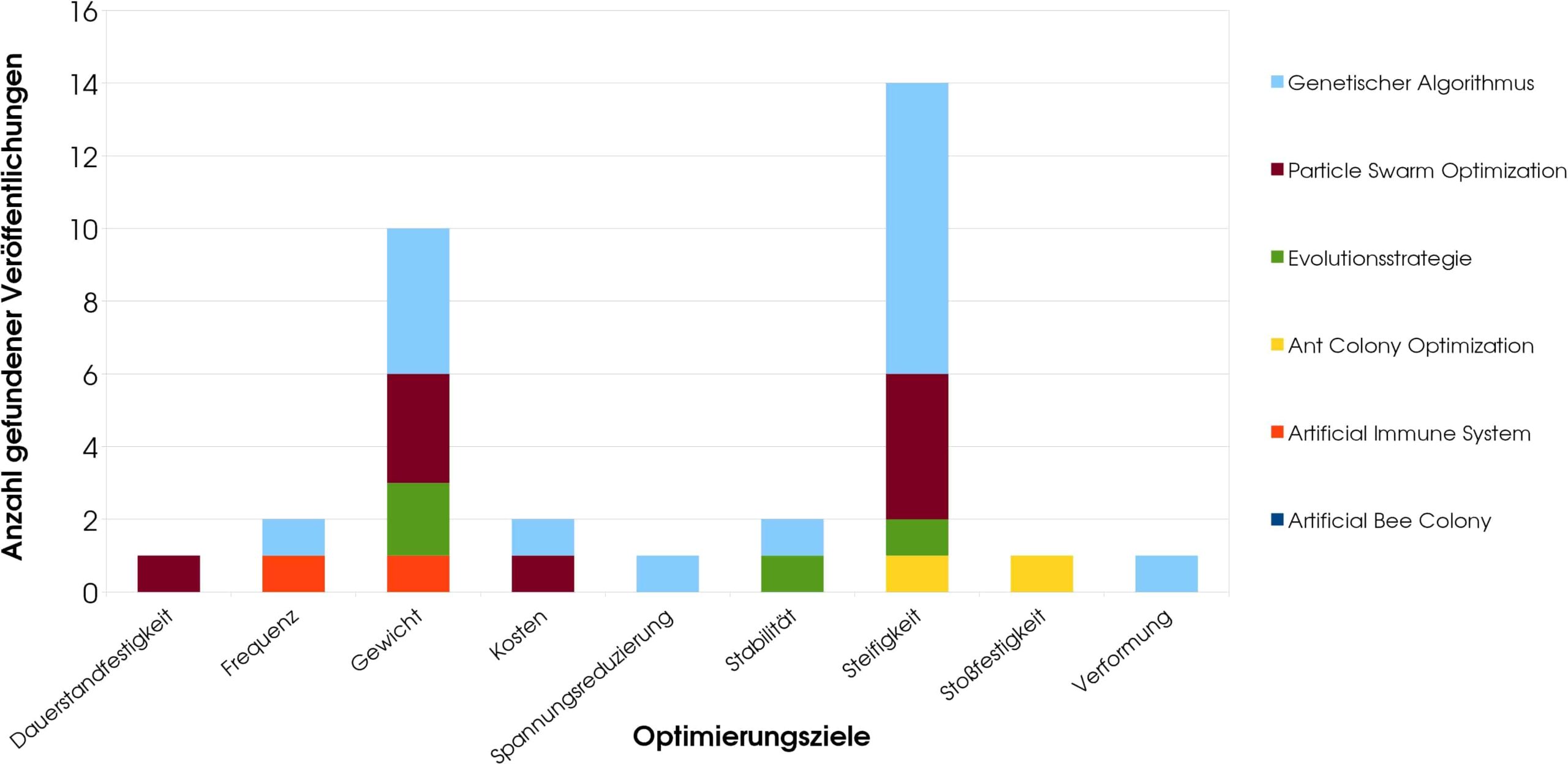
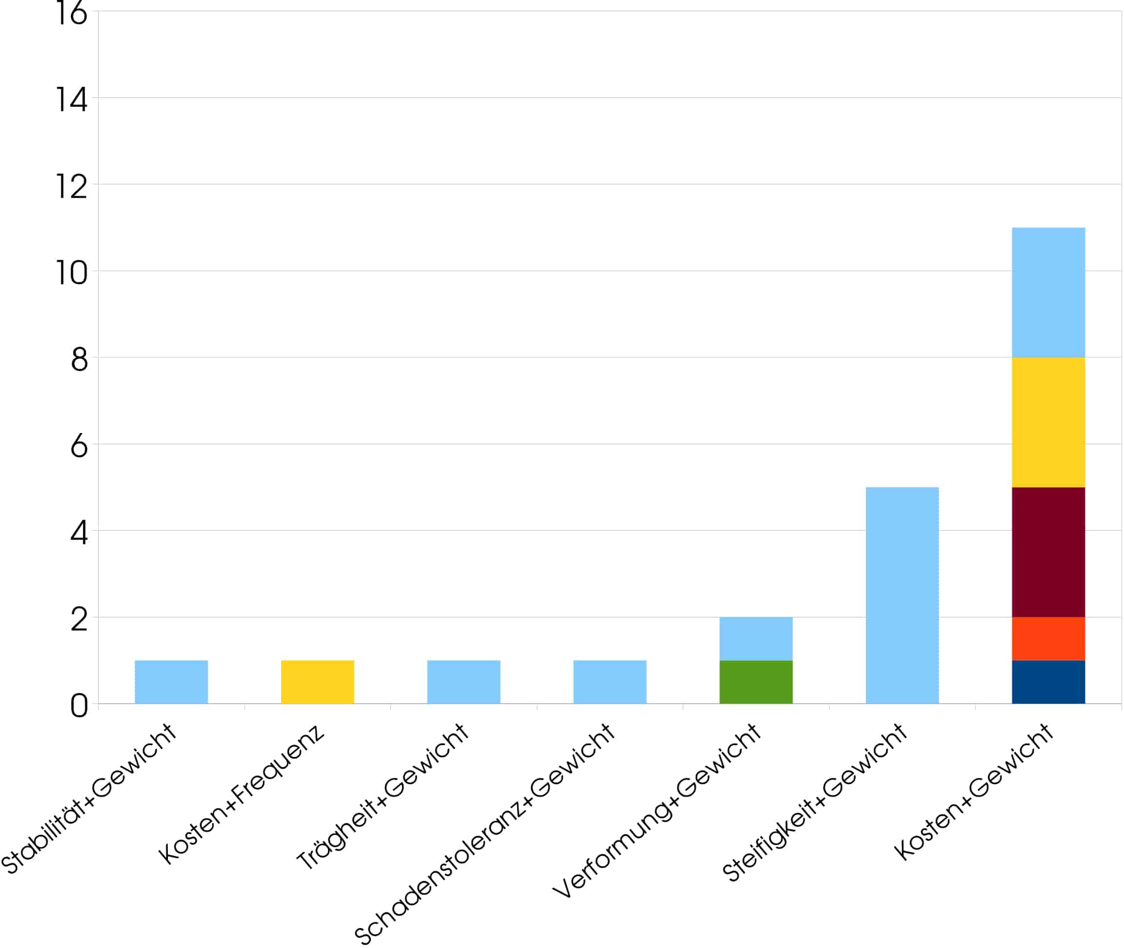
A total of 56 publications were found that each applied one of the optimization methods mentioned. The optimization objectives here were: fatigue strength, frequency, weight, cost, stress reduction, stability, stiffness, impact resistance, deformation, and, applied once each in multi-objective optimization, inertia and damage tolerance. These optimization goals are typical for the field of mechanical engineering and therefore not surprising. The frequency of the algorithms used varies greatly, which is also not very surprising. In simple optimization, the goals of stiffness and weight dominate, which is plausible given that this is a lightweight construction technology. It was not to be expected that the objective of cost would receive little attention, since high costs are one of the greatest challenges in the manufacture and processing of fiber composites. In multi-objective optimization, however, the situation is different; here, cost, together with weight, is the most frequently used of all optimization objectives. Stiffness and weight are the second most frequently used. The remaining combinations of objectives are marginal in comparison to these two.
In addition to the frequency of use of the optimization goals, it is important to look at the frequency of use of the individual algorithms. With 29 applications, GA is by far the most widely used. PSO follows far behind with 12 applications, ACO with 6, ES with 5, AIS with 3, and ABC with a single application. Table 2 also lists the year of origin and the degree of familiarity (according to our own assessment). The fact that GA is used so frequently is mainly due to its high profile; GA is so popular that it is now even used synonymously for any nature-analogous algorithmic optimization, and most engineers, even those who have no connection to algorithmic optimization, are at least familiar with the term. Two other things stand out: First, it’s interesting that PSO is the second-newest algorithm of all the ones covered here, but it was already the second-most used. Second, it is striking that ES, which together with GA was the first nature-inspired optimization algorithm ever, has been used only very rarely. The fact that the developers failed to popularize ES has meant that today it is best known in Germany, where it originated. However, ES does not need to hide behind the other methods, because on the contrary, it is actually a big step ahead of them: it has already been intensively studied by mathematicians, engineers, and computer scientists, and its performance has been repeatedly confirmed, see [3], [4], among others. This is where the “underdog” has its chance, namely that it is little known, but at the same time has one of the most solid foundations of all.
| Algorithm | Newness (Establishment) | Popularity (+/-) | No. found publications |
|---|---|---|---|
| GA | 1970 | + | 29 |
| PSO | 1995 | – | 12 |
| ACO | 1992 | – | 6 |
| ES | 1970 | – | 5 |
| AIS | 1994 | – | 3 |
| ABC | 2005 | – | 1 |
Laminate optimization
Selection of the optimization algrithm
One of the available methods mentioned in Chapter 4 is now selected and used to optimize the laminate. In this work, the Evolution Strategy is chosen because
- it has been comprehensively developed and investigated using scientific and empirical methods
- it has been refined and further developed over more than 40 years of research
- it has rarely been used for laminate optimization to date, which is due to its lack of recognition but does not do justice to its potential
- evolution is an overarching principle that explains most other natural biological mechanisms that have been transferred to optimization processes.
Operating principle of the Evolution Strategy
The Evolution Strategy is a heuristic. Heuristics are used at the latest when deterministic methods can no longer deliver satisfactory results due to overly complex problems. The ES adopts the principle of evolution, specifically that of Charles Darwin.
This study uses (μ/ρ +, λ)-ESs (pronounced “mu over rho plus comma lambda evolutionary strategies”). Here stand
- μ for the number of parents
- λ for the number of children
- ρ for the number of an recombinants, that means the number of parents that recombine from which a child emerges (in nature it is with few excemptions equal 2).
In addition, a starting step size σS must be specified. Based on the current starting configuration, μ new solutions are now generated by varying the variables. The variation is normally distributed with σS as the dispersion measure and 0 as the mean. In the next step, the children are generated. If ρ=1, or with certain other parameter settings, the parents generate the children by simply copying themselves. Any differences in the child are then generated solely by mutation of its genes. For ρ≠1, the child consists of mixed parent genes, which are then additionally mutated. At this point, there is a generation consisting of μ parents and λ children. The objective function is now evaluated for all parents and children (which in this work represent laminates with different angle settings).
The next step is selection, which corresponds to the principle of “survival of the fittest” in biological evolution. First, a distinction must be made between the strategy types, i.e., between (+) strategy and (,) strategy. It is therefore a binary input parameter. In a (+) strategy, the objective function values of the existing parents and children are compared with each other. Those μ of them with the best target function values are selected as parents for the new generation. In a (,) strategy, exactly the same thing happens, with the crucial difference that only the children are selected as the new parents. In (,) strategies, the parents of one generation cannot be selected as parents for the next generation and participate again in the creation of new children. For (,) strategies, this requires an input of λ ≥ μ; this restriction does not apply to (+) strategies.
In addition to selecting new parents, something else very important happens: the step sizes are adjusted. It is not practical for subsequent generations to also vary according to the start step size; instead, it must be continuously adjusted throughout the optimization process. This can happen in various ways. In this work, two well-established mechanisms are used, namely the 1/5 success rule and one that controls individual step sizes, referred to here as the “τ rule.” The 1/5 success rule is only applicable to (+) strategies; furthermore, recombination cannot be implemented when it is used. The τ rule, on the other hand, can be used for both strategy types and also with recombination. See also Chapter 6.5 and Fig. 6. The reasons for these different areas of application are historical. (+) strategies were the first evolutionary strategies; the 1/5 success rule was developed at this stage. (,) strategies and the possibility of recombination were developed later, and in this context, the τ rule was also developed. A good, sufficiently detailed summary of how both step size control mechanisms work can be found, for example, in [7].
The process described in this chapter continues over several generations, i.e., iteration steps. At the end of the optimization, depending on whether minimization or maximization is used, the parent with the lowest or highest function value represents the optimal result. For more detailed information on the Evolution Strategy, see [4], [5], [6], [7], [8], [9], [10], among others.
Optimization criterias
In order to optimize, a system must be defined. This is the initial configuration. When optimizing laminates with variable angles of the individual layers, the initial configuration is an arbitrarily selectable angle arrangement. Furthermore, variables that can be varied must be specified (so-called “design variables”). In this case, these are the orientations of the individual layers. Since this is a discrete optimization problem due to the specification of discrete angles, this set of angles must also be specified. Finally, an objective function is established that must be minimized or maximized. The objective function in this work is to minimize the maximum stress fE of the associated failure mode according to the CUNTZE failure criterion. For this purpose, the stress state and all 5 failure modes are evaluated for each currently set laminate configuration (i.e., the angles of the individual layers). The failure mode that assumes the most critical and thus highest value determines the objective function to be minimized. The optimization task therefore formally consists of finding the optimal angle configuration for which the maximum stress of the most stressed layer is minimized. This expresses the optimization of the alignment of all layers and thus of the entire layer structure.
Of particular interest in this work is how the parameter settings of the Evolution Strategy affect the quality of the result and which parameter configuration is suitable for which number of layers. Since heuristic optimization is highly probabilistic, exactly 100 optimizations are performed in this work for each parameter setting and number of layers. The averaged result then provides reliable information about how well the parameter setting was chosen. The quality of the result is evaluated based on two characteristics: The most important evaluation criterion is the number of successful optimizations, i.e., reliability. A success rate of 80% is specified in this work. At least 80% of the 100 optimizations must not deviate more than 10% from the global optimum (i.e., be greater than 1.1, see Chapter 6.4). In addition, care is taken to ensure that the average number of function evaluations remains low. The number of function evaluations is a measure of the speed and computing capacity required by the algorithm. Of all parameter configurations, the best one is ultimately the one that achieved/exceeded the success rate and required the fewest function calls on average.
Problem formulation
The layers of the laminate can be fixed in a rotatable manner, which in this work are also the variable parameters of optimization and often represent one of the few free variables in laminate design. However, since it is rarely possible to realize all angles in industrial series production, a set of discrete angles is generally used. In this model, the following set of possible angles is defined:
{0°, 15°, 30°, 45°, 60°, 75°, 90°, 105°, 130°, 145°, 160°, 175°}
The orientation of a UD layer can therefore be varied in 15° increments in the range between 0° and 180°. The range between 180° and 360° inclusive does not need to be defined, as the property profile of a standard UD layup has two planes of symmetry, meaning that an orientation of 270°, for example, corresponds to an orientation of 90°.
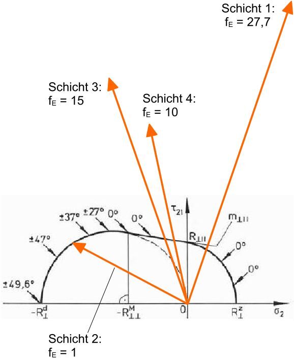
There are basically two ways to determine a starting configuration from which optimization can be performed: One option is the one that is used in practice in the vast majority of cases, as there is little or no evidence for a good initial configuration from which the optimum could be found with a high degree of probability. This first option is to determine the starting configuration completely arbitrarily, i.e., at random. The other option is to make it as difficult as possible for the algorithm and specify the worst possible configuration in order to simulate the singular case of a completely unsuccessful starting configuration. This second option is used in this work, rotating the entire laminate by 90° so that the load acts orthogonally to the fibers. The value of the objective function in this configuration is 27.7. Although there are other configurations that assume even worse objective function values (e.g., complete laminate rotation by 75° and 60° with maximum effort of 28.19 and 34.60, respectively), but since the starting point is furthest from the optimum due to a 90° rotation, it is still behind these additional maxima that must be overcome.
This allows us to subject the algorithm to the most rigorous stress test possible. This means that the objective function landscape must be overcome in the most difficult way possible and by the longest possible route. Those results that achieve the specified quality measure can be regarded as outstanding achievements of the algorithm when one considers that we started from the singular “worst case” and that the objective function is discontinuous and partially non-differentiable (discrete changes in the CUNTZE fracture mode and the relevant single layer).
In this work, a specific and constant load case will be applied for which the solution is known. The laminate model under consideration in this work is subjected to uniaxial tension in the longitudinal direction and also to a bending moment about the axis in the fiber direction. With regard to CUNTZE failure, the stress situation considered here is normalized in such a way that, with optimal orientation (when all layers are aligned at 0°), the fracture condition is just satisfied and the stress assumes its permissible maximum value, which is f0 = 1.
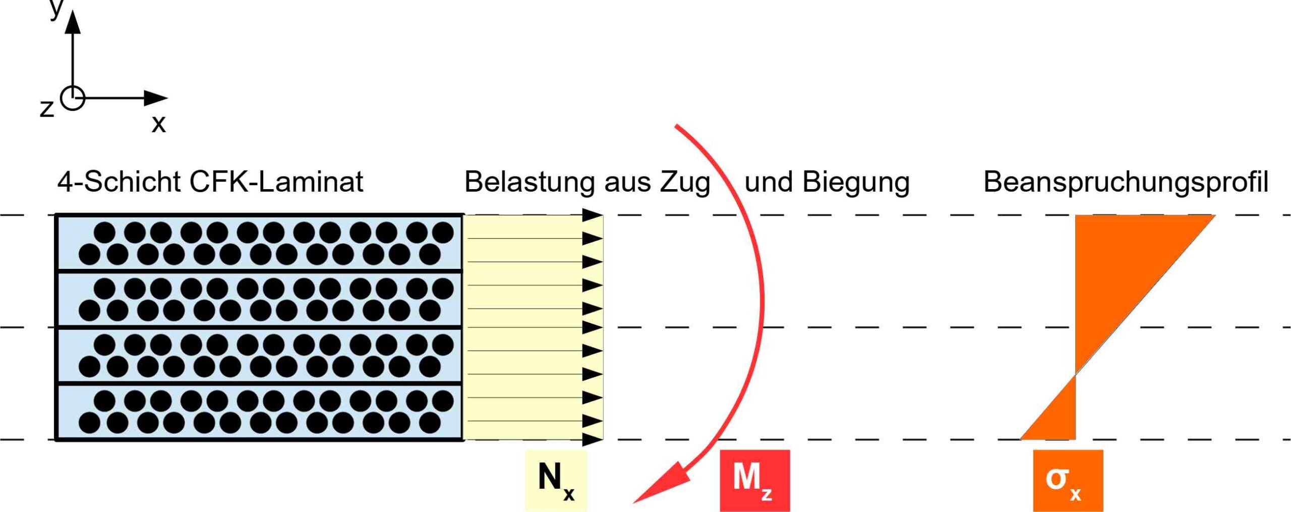
This load profile places the greatest stress on the top layer. This is deliberately chosen so that the layers are not symmetrical and therefore not subjected to the same load, which could cause redundancy effects in the optimization that would interfere with the evaluation and assessment. The fact that a certain layer or certain layers are subjected to greater stress than others also allows attention to be focused on how the algorithm deals with the resulting differences in sensitivity. Rotating the top layers therefore has a significantly greater influence on the objective function than the lower layers. However, the algorithm should not stop once it has rotated the most heavily stressed layers into the correct position, but should also correct the layers that have a comparatively lower sensitivity to the objective function.
First, a good parameter setting is sought for a laminate with a layer count of 4. A low number of layers ensures that it is possible to experiment with many parameter settings in a relatively informal manner at low cost, as the computing time generally remains moderate. Once you have familiarized yourself with how the system responds to different inputs, which inputs have a greater influence on the target function than others, and how fast and reliable the optimization is with individual parameter configurations, the laminate is scaled up. This is done by increasing the number of individual layers to 8 and then 12. The findings from the optimization of the 4-layer laminate should serve as a guide and support for higher-scaled laminates, although it must be borne in mind that the objective function changes significantly with a significant increase in the number of layers. It becomes not only quantitatively more complex due to the increasing number of possible angle configurations, but also qualitatively more differentiated and highly modal (more local optima). This makes it necessary to redefine the parameter configuration each time.
Parameter studies
This optimization model has a total of 9 input parameters:
- Number of parents: μ ∊ ℕ>0
- Number of children: λ ∊ ℕ>0
- Strategy type: (+) oder (,)
- Start step size: σS ∊ ℝ>0
- Mutative step regulation (MSR): 1/5 success rule or τ rule
- MSR-parameter of τ rule: τ1 and τ2 ∊ {0,1} ∊ ℝ
- Number of recombining parents: ρ ∊ {1,μ} ∊ ℕ
- Termination criteria ε ∊ {0,1} ∊ ℝ>0
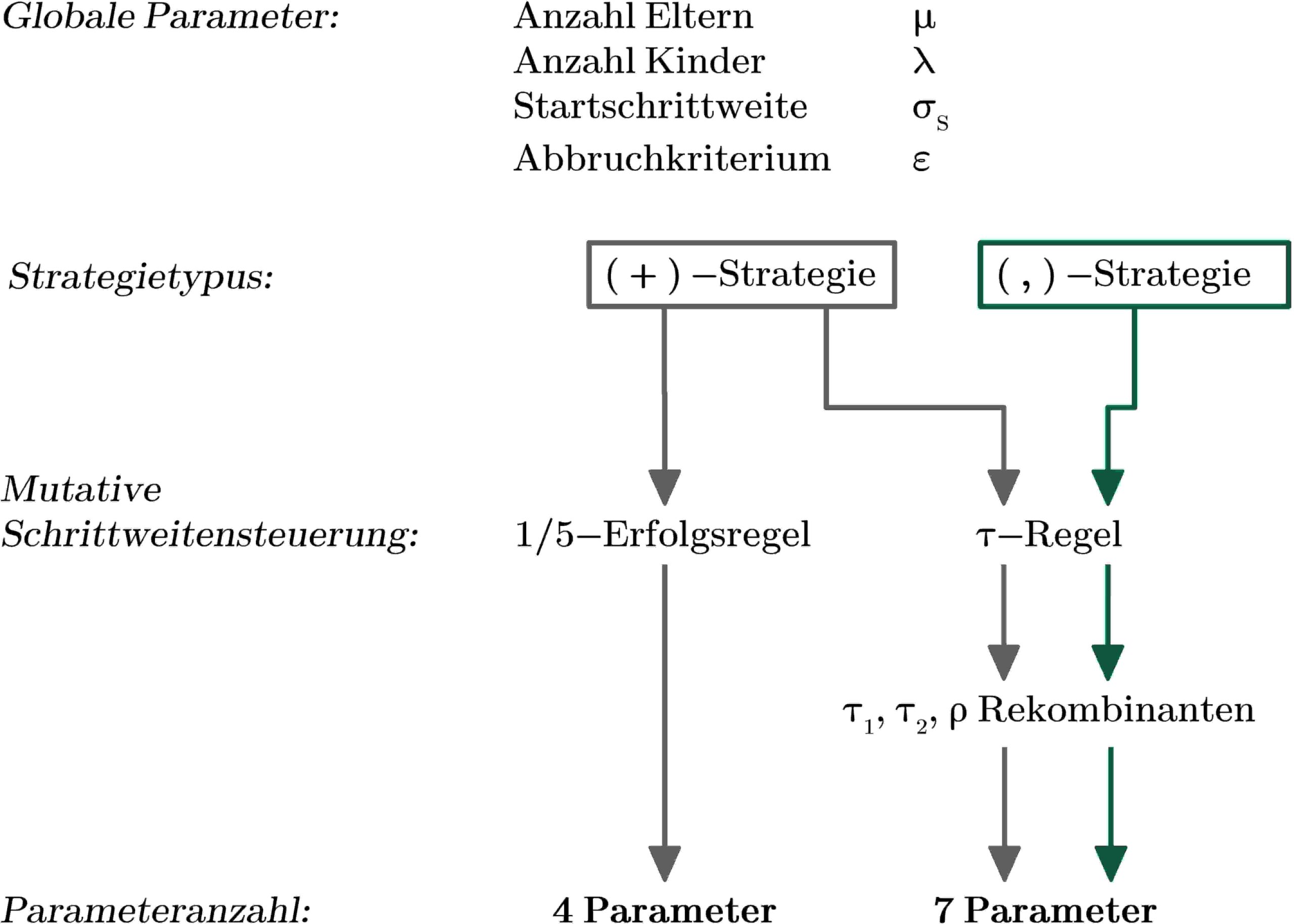
However, not all parameters for optimization need to be entered; they depend on the strategy and are interdependent. For example, depending on which MSR is used, a (+) strategy has exactly 4 or 7 input parameters, while all (,) strategies always have exactly 7 input parameters.
The parameters have varying degrees of influence on the optimization process and fulfill different tasks. Some are global and overarching, while others are very specific to sub-functions. They cannot be considered equal in terms of their importance in fulfilling their tasks or their degree of influence on the optimization process and thus its result.
The set of 9 global input parameters has value ranges that are mostly infinitely large (real numbers in general or integers without upper limits). Of several different and noteworthy approaches, this paper chooses to work initially with (+) strategies and the 1/5 success rule as MSR for two reasons. With such an ES, there is the smallest number of possible input parameters, which is why it can be used to create a good first draft of a parameter configuration. Furthermore, it can help to make statements about the nature of the objective function, which will be useful for the parameter settings of other ESs. For example, the convergence behavior of a (1+1) ES with low start step sizes can be used to explore the immediate vicinity of the objective function starting from the initial configuration. If a local optimum is found after a few iterations, this provides information about its existence (it exists), its characteristics (function value can be reproduced), and its approximate distance (close).
The more complex the objective function is, e.g., noisy and highly modal, the more the (+) strategy is inferior to the (,) strategy in finding global optima, but superior in terms of speed and convergence reliability, which are further reasons to consider it first.
The 1/5 success rule is the older of the two MSRs and has gained considerable fame due to its striking nature (“on average, exactly one successful mutation out of five”) and, no less importantly, due to its scientific elaboration and justification. It is also of interest in this work because, when it was developed over 40 years ago, it was one of the earliest self-adaptive mechanisms and has remained unchanged to this day.
The complexity of both strategy types, (+) and (,), is the same when using the other MSR, the τ rule. Nevertheless, the next step will continue to use the (+) strategy in conjunction with the τ rule, because (+) strategies are faster than (,)-strategies. As long as at least 80% of successful optimizations can be achieved with a (+) strategy, a (,) strategy is not necessary and will usually take longer. Only when success can only be achieved with very large parameters using the (+) strategy, or conversely, when this takes a disproportionately long time, will (,) strategies be used in this work.
The number of parameters to which one is exposed when the 1/5 success rule does not apply is too large to be able to give them all equal attention. Of central importance are the three overarching variables that are used in every strategy: the number of parents, the number of children, and the start step size. There are generally few recommendations or guidelines to follow for these parameters. Their most important meanings are as follows: The more parents are generated, the greater the probability of finding the global optimum, but this comes at the expense of speed. The larger the number of children selected, the more reliably the algorithm converges, but this also comes at the cost of a more complex procedure. A recommendation for setting the ratio of parents to children is given in [6], according to which it should be around 1:7. This serves as a guide in this work; however, there will also be significant deviations from it. The following applies: The smaller this ratio is, the greater the “selection pressure.” High selection pressure means that there is little tolerance for inferior solutions. In practical terms, this means that convergence reliability and speed increase with increasing selection pressure, but the probability of finding the global optimum decreases. The more benign the system to be optimized is, the more permissible high selection pressures are. See also [7] for more information.
Well-adjusted start step sizes depend largely on the starting point, the nature of the objective function, and the overall constitution of the system. They should be based on the size of the design variable vector, as they must be proportional to this. In this work, the vector has a length of 12 (0° 15° 30° 45° …). It therefore makes little sense and has little chance of success to choose starting step sizes of around 10 to 12 or 0.1 to 0.7. The former spans almost the entire vector, causing the normal distribution to degenerate into a uniform distribution, and the latter does not take the vector length into account, causing too many elements to be ignored at the beginning of the optimization. In particular, since the worst possible configuration is used as the starting point, it is crucial to have sufficiently large step sizes at the beginning. In this work, integer starting step sizes between 1 and 8 will be used.
When applying the τ rule, three factors need to be defined: τ1, τ2, and the number of recombinants ρ.
Although it would be interesting to investigate the influence of the parameters τ1 and τ2, this will not be done in this study, apart from a few tests. On the one hand, this is because τ1 and τ2 have little influence and have only a minor effect on convergence behavior, speed, and reliability. Secondly, these two variables are exceptions in the parameter pool of ESs in that recommendations have been made for them in the specialist literature, which are used in this work. For example, [6] recommends setting both between 0.1 and 0.2. In this work, τ1 is set to 0.1 and τ2 to 0.2.
In contrast, an important factor is ρ, which is a measure of the mixing of individuals. If no recombination takes place, i.e., if ρ is equal to 1, the parent generates a child from itself with a modified configuration according to the current step size and the normal distribution. When parents (two, as is known from nature, or up to all available) cross, their configurations are first mixed completely randomly and then varied as above according to the step size and normally distributed probability. In this work, ρ will essentially be used with three settings, namely
- 1, whereby the quality of crossbreeding should be abstracted in general,
- 2, to represent the usual “natural” crossing, and
- μ, which marks the extreme value.
The termination criterion ε is the ratio of the fitness (meaning: value of the objective function) of the best of a generation to the mean fitness of all parents and children of that generation. It is commonly set between 0.7 and 0.99, depending on various factors. The most important factor is to check how many optimizations in a 100-time study reach the global termination threshold of 80 generations specified here. If it is reached, it is classified as not converged. However, if good results still emerge, it can be assumed that the termination criterion is set too leniently. After readjusting and correcting it in these cases, the good results usually remain, while the number of generations required decreases. ε is therefore a parameter that is initially set high (e.g., 0.95 or 0.99). If the results are good but various to many optimizations take time to reach the global termination threshold, ε is then scaled down for the next attempt with otherwise identical parameters. In this way, the ratio of successful, valid optimizations per study and low function evaluations required is balanced.
Results
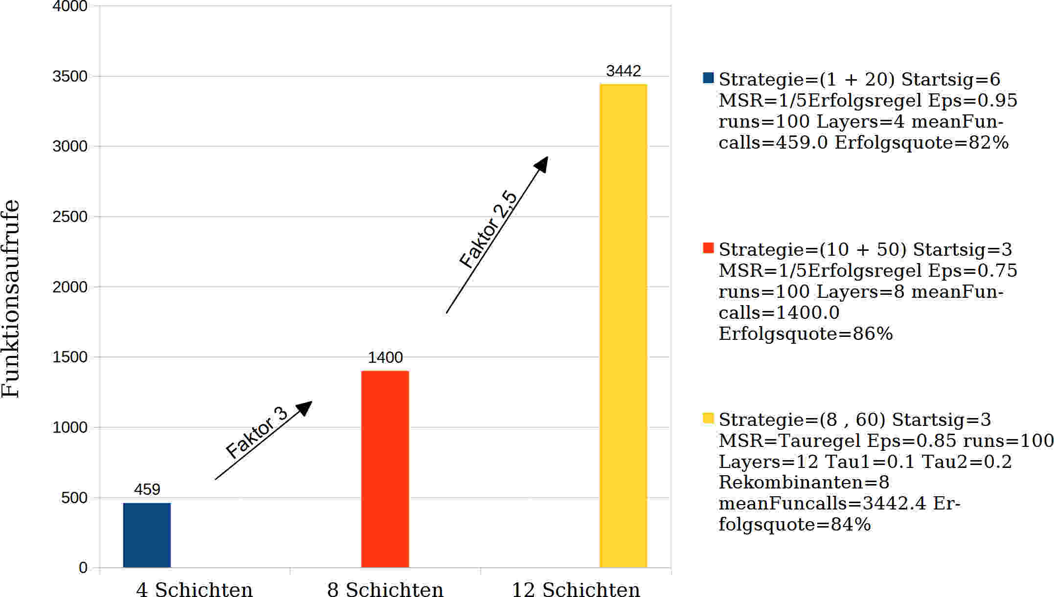
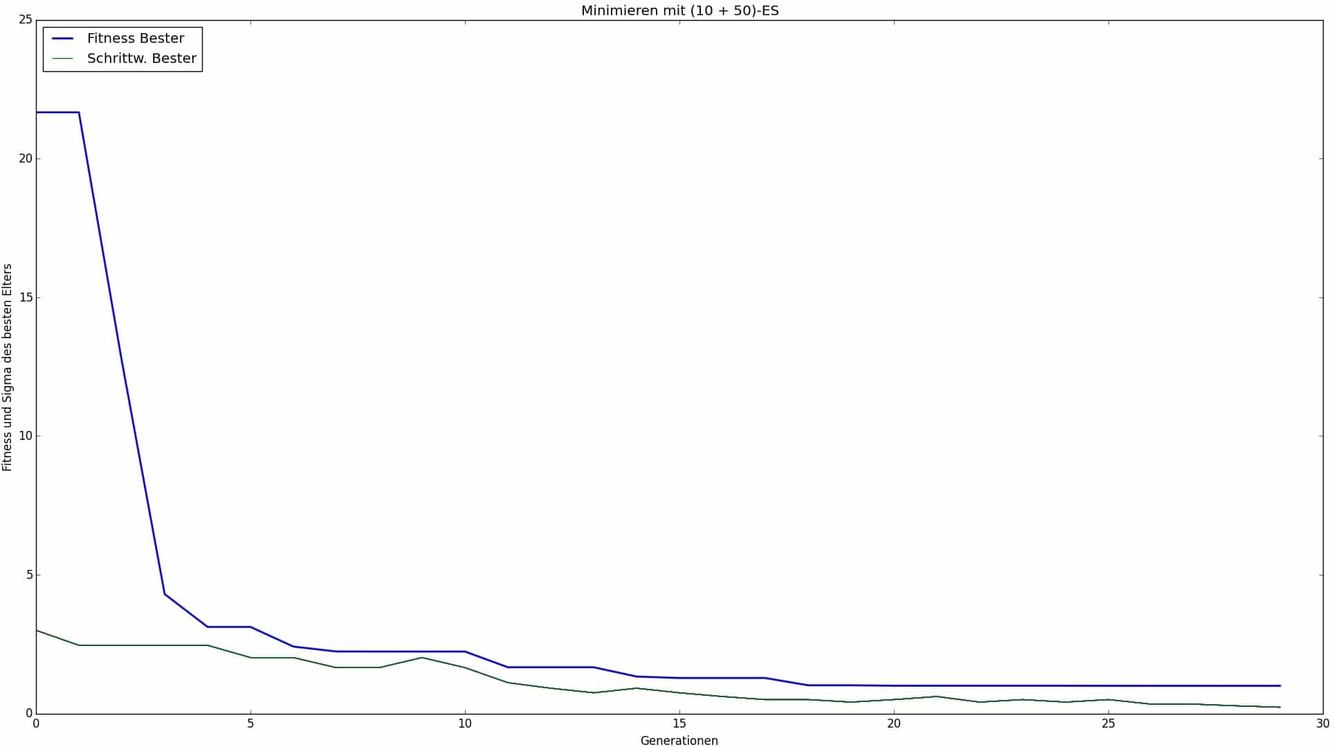
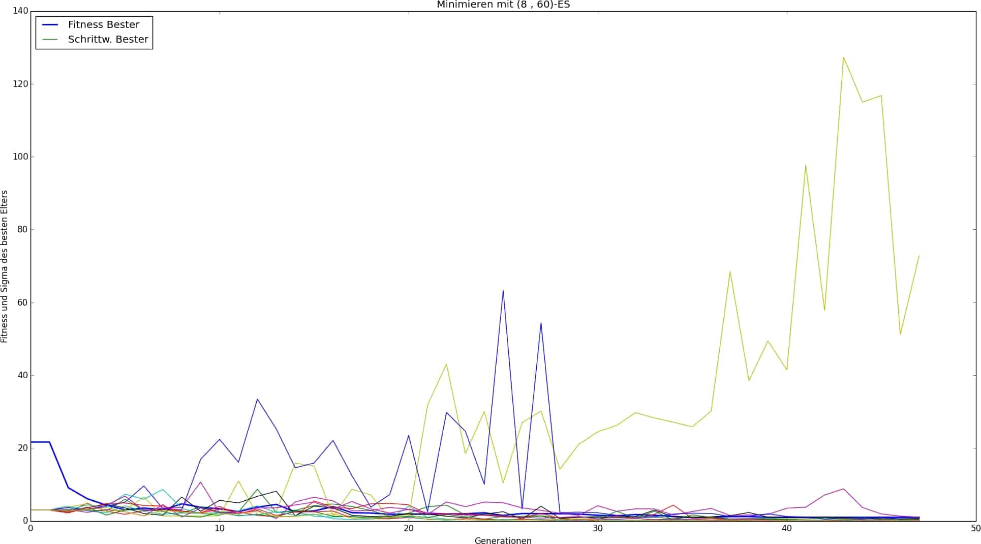
Following the procedure described above, results were obtained which are summarized in Table 3 and Table 4 as well as in Fig. 7.
| Parameter | 4 layers | 8 layers | 12 layers |
|---|---|---|---|
| Strategy | (1 + 20) | (10 + 50) | (8 , 60) |
| Start step size σS | 6 | 3 | 3 |
| MSR | 1/5 success rule | 1/5 success rule | τ rule |
| τ1 | – | – | 0,1 |
| τ2 | – | – | 0,2 |
| Recombinants ρ | – | – | 8 |
| Termination crit. ε | 0,95 | 0,75 | 0,85 |
| Parameter results | 4 layers | 8 layers | 12 layers |
|---|---|---|---|
| Average number of function calls | 459 | 1400 | 3442 |
| Average required generations | 24 | 29 | 58 |
| Average functional value | 1,18 | 1,095 | 1,07 |
| Average computation time | 0,8s | 4,3s | 30s |
| Number of not converged optimizations | 0 | 0 | 13 |
| Success quota | 82% | 86% | 84% |
When determining the parameters, it was recognized, as expected, that the setting of the start step size has a very large influence on the result. Start step sizes greater than 4 and smaller than 3 were generally not useful in the experiments. The 4-layer laminate with the best start step size of 6 is an exception. In all other cases, the success rate decreased with start step sizes greater than 4 and less than 3, with increasing deviations.
Furthermore, significantly better results were recorded for the 4- and 8-layer laminates using the 1/5 success rule than using the alternative τ rule, both for (+) and (,) strategies. Strategies using the 1/5 success rule also achieved good results for the 12-layer laminate. In most cases, they even found the optimum with reasonable runtime (i.e., reasonable number of average function calls required) much more reliably. It should be noted that deviations from parameter settings were relatively robust and benign with regard to the results, which is to be considered positive. Of all three strategy types/MSR combinations, (+) strategies using the τ rule performed the worst. Although the quality of their results is usually good, the algorithm shows major convergence problems. This is due to the fact that it is problematic to apply the τ rule to (+) strategies as it can fail here. See Chapter 8 for more information.
Despite the good results achieved for the 12-layer laminate using (+) strategies in combination with the 1/5 success rule, the best result was achieved for this laminate using a (,) strategy. This was to be expected given the nature of (,) strategies, which are designed for difficult objective functions. Since it can be assumed that the complexity of the objective function of a laminate increases at least exponentially with the number of layers, this justifies and ultimately necessitates the use of (,) strategies to the same increasing extent.
The factor of recombination has proven to be extremely significant. Strategies without recombination, i.e., with ρ=1, generally had the worst results, strategies with ρ=2 had significantly better results, and strategies with ρ=μ had by far the best results per configuration. However, this was only possible if the number of parents and children and the start step size were set appropriately. As has also been shown, a recombination factor of ρ=μ cannot compensate for insufficient settings of these variables. It should be noted, however, that in this work, experiments were only carried out selectively beyond a parent number of μ=10. The validity of the observations beyond this number is no longer given or is only given to a limited extent.
With regard to the selection pressure for the laminate optimization studies conducted here, it has been found that good results were actually achieved with a sufficient population size and a parent-to-child ratio of 1:7, as recommended in [6]. This is also recommended as a guideline for laminate optimization.
With regard to the termination criterion ε, it has been found that its optimal setting does not depend, or at least only secondarily, on the number of layers, but that it is strategy-dependent and must be reset for each new strategy. This finding is also plausible, since the nature of the objective function and, in particular, the optimum also influence the convergence behavior of the strategy. However, the population behavior, in general and in the vicinity of the optimum, varies from strategy to strategy, which requires ε to be readjusted each time. No regularity can be derived from this.
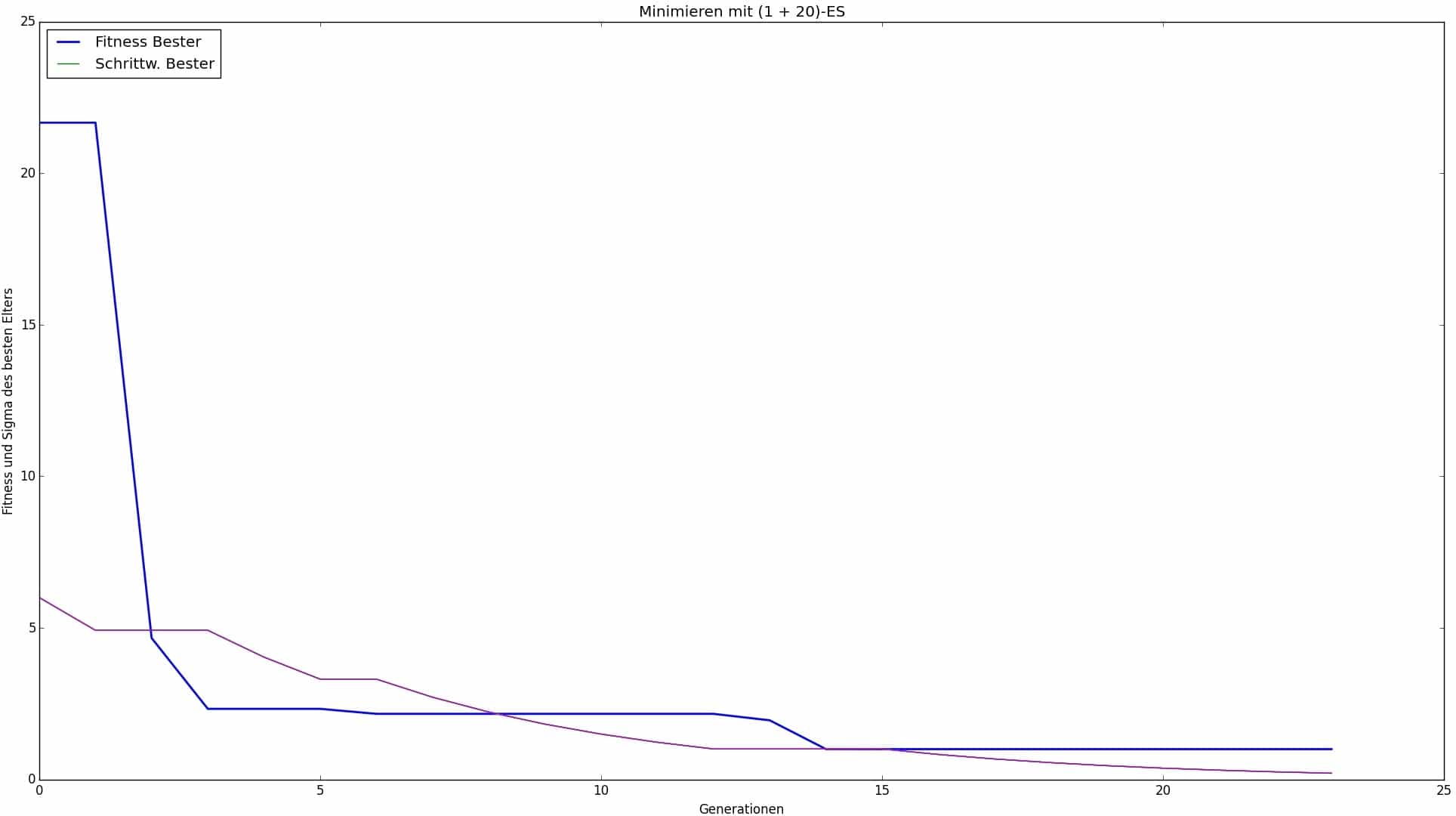
Fig. 8: Optimization of a 4-layer laminate with parameters according to Table 3
Discussion
First, it should be noted that these investigations into laminate optimization are a worst-case scenario, for which a catastrophically failed laminate design was used as the starting configuration. Therefore, significantly better results and more benign behavior of the algorithm in response to parameter inputs can be expected when starting with a randomly generated initial configuration, as is common practice. The important maxim that a sufficiently good initial configuration must be available in order to fully exploit the potential of the optimization process was deliberately strained in this work. In addition to the laminate optimization that was carried out, this measure also served as a performance test of the algorithm.
The results show that for low numbers of layers, the (+) strategy in conjunction with the 1/5 success rule is perfectly adequate and even delivers by far the best results and converges most reliably. The good news for users is that it also requires the fewest parameters to be entered, meaning that it is difficult to go wrong with it in the low-number multi-layer compounds examined here. It is definitely permissible and recommended to start with only one or a few parents and a relatively large number of children, as this already yields remarkable results.
The choice of the start step size is crucial and must be matched to the length of the vector carrying the design variables. In this case, the design variable vector was the one containing the angles and therefore had a length of 12. Successful start step sizes were therefore 3 and 6, which correspond to 25% and 50% of the length, respectively. This is recommended as a guideline for optimizing higher-scaled laminates as well as for design variable vectors of greater or lesser length. In case of doubt, smaller starting step sizes are preferable, since with a random starting configuration, all layers are usually closer to the optimum than was the case in this work. The fact that the start step sizes determined here are in the left to middle range of the vector is due to the fact that the optimum layer angle, which was known in this work and was the same for all layers (0°), was slightly further to the left of center in the implementation. Since the optimal angles are not normally known and can be located at any point in the vector and at different points for each individual layer, this does not represent a rule.
(,)-strategies are significantly less convergence-safe and more sensitive in terms of the settings to be made. This has been confirmed in this work. (,)-strategies should generally be avoided for low-number multilayer composites. They play to their strengths in cases of high complexity, but this comes at the price of high sensitivity in terms of optimization time, convergence reliability, number of parameters, and parameter influence. This can be seen, for example, in the 12-layer laminate with settings according to Table 3, whose optimization process is shown in Fig. 10. The fact that two step size values deviate significantly from the one that is no longer reduced until termination is an indication that the convergence behavior is unstable. It should be noted that the convergence behavior for a specific (and this) strategy could be improved by fine-tuning all parameters. However, this would only be of cosmetic significance here, as the results achieved are completely satisfactory.
(+) strategies using the τ rule were the most problematic of all those considered in this work. They converged only very rarely, which is also due to their structural weakness. This is also highlighted, for example, in [7]. This weakness can be described figuratively as follows: If, for example, a parent has a relatively good quality, it is close to a local optimum. If it creates children from there with currently relatively large step sizes, but there are no better function values available at this distance, these are then practically never selected (as they always have poorer qualities). Furthermore, the step size of the parent no longer adapts (which would happen by creating a more successful child and would result in the replacement of the parent). The result is virtually infinite and unsuccessful progress. However, it is still possible to work with (+) strategies using the τ rule. To use them, a different termination criterion than the one defined here must be specified. For example, it makes sense to terminate after a certain number of generations or after a certain number of generations in which there has been no improvement (i.e., replacement) of the best. To compensate for their structural deficit, it is advisable to operate with a high number of children in order to increase the probability of breaking away from relatively low-value positions. Furthermore, small rather than large initial increments are recommended.
The factor that reflects the increased computing effort with increasing number of layers and optimal settings according to Table 3 is between an 8-layer and a 4-layer laminate with 1400 function calls / 459 function calls = 3. The factor between a 12-layer and an 8-layer laminate is 3442 function calls / 1400 function calls = 2.5. In contrast, the factor reflecting the increase in possible angle configurations and thus also possible solutions from 4 to 8 and from 8 to 12 layers is 128 / 124 = 1212 / 128 = 124 = 20736.
This clearly shows that evolutionary strategies and simply varying parameter settings can be used to master enormous increases in complexity and degrees of complexity. It is therefore expressly suitable for laminate optimization and should also be considered for other complex optimization tasks involving FRPs.
Literature
[1] Schürmann, Helmut: Konstruieren Mit Faser-Kunststoff-Verbunden. 2. Aufl.. Berlin Heidelberg New York: Springer-Verlag, 2007.
[2] Cuntze, R. u.A.: Neue Bruchkriterien und Festigkeitsnachweise für unidirektionalen Faserkunststoffverbund unter mehrachsiger Beanspruchung: Modellbildung und Experimente; BMBF-Förderkennzeichen 03N8002; Abschlußbericht 1997. Düsseldorf: VDI-Verlag.
[3] Born, J.: Evolutionsstrategien zur numerischen Lösung von Adaptionsaufgaben; Dissertation an der Humboldt-Universität, Berlin, 1978.
[4] Bäck, Thomas; Foussette, Christophe; Krause, Peter: Contemporary Evolution Strategies. 1. Aufl.. Berlin Heidelberg: Springer Science & Business Media, 2013.
[5] Rechenberg, I.: Evolutionsstrategie ’94. Stuttgart: Frommann-Holzboog, 1994.
[6] Nissen, V.: Einführung in Evolutionäre Algorithmen: Optimierung nach dem Vorbild der Evolution. 1997. Aufl.. Wiesbaden: Vieweg+Teubner Verlag, 1997.
[7] Kost, B.: Optimierung mit Evolutionsstrategien: eine Einführung in Methodik und Praxis mit Visualisierungsprogrammen. 1. Aufl. Frankfurt am Main: Deutsch, 2003.
[8] Harzheim, Lothar: Strukturoptimierung: Grundlagen und Anwendungen. 2. Aufl. Haan-Gruiten: Europa Lehrmittel Verlag, 2014.
[9] Beyer, Hans-Georg: The Theory of Evolution Strategies. 2001. Aufl.. Berlin Heidelberg: Springer Science & Business Media, 2001.
[10] Schöneburg, Eberhard; Heinzmann, Frank; Feddersen, Sven: Genetische Algorithmen und Evolutionsstrategien: eine Einführung in Theorie und Praxis der simulierten Evolution. Amsterdam: Addison-Wesley, 1994.